Correspondence with web applications
By using page_type, we can make it compatible with the web application (https://aiphad.org/).
Using this option, it is possible to obtain the figures of predicted phase diagrams and uncertainty scores.
page_type is specified as follows.
pdc  = pdc_sampler(page_type = "ternary_section",
                   input_data = "data.csv",
                   estimation = "LP",
                   sampling = "LC",
                   proposal = 1
                   )
The page_type that can be specified here is as follows.
“two_variables”: Diagrams with 2 variables
“three_variables”: Diagrams with 3 variables
“ternary_section”: Phase diagrams for ternary section
“ternary”: Phase diagrams for ternary
“quaternary_section”: Phase diagrams for quaternary section
When inputting a csv file to input_data,
we need to use a file that corresponds to the one specified in page_type.
Example for ternary section
Here, as a basic example, we will explain using the case of the ternary section (“ternary_section”).
We specify “ternary_section” for page_type to investigate the phase diagram of a ternary isothermal section.
In this example, the input is given as a csv file and the figure is output to the screen.
Import modules are as follows. We can visualize the phase diagram by importing aiphad.aiphad_output.
from aiphad import pdc_sampler
from aiphad.aiphad_output import plot_out
import numpy as np
The python code is written as follows:
pdc  = pdc_sampler(page_type = "ternary_section",
                   input_data = "data_ternary_section.csv",
                   estimation = "LP",
                   sampling = "LC",
                   proposal = 5
                   )

pdc.fit()
pdc.us()
plot_out(pdc)

proposals_index = pdc.proposals
proposals_X = pdc.proposals_X
proposals_us = pdc.proposals_us

print("proposal_index:", proposals_index)
print("proposal_X:", proposals_X)
print("proposal_us:", proposals_us)

belonging_index = pdc.belonging_index
belonging_X = pdc.belonging_X
belonging_probability = pdc.belonging_probability

for key, value in pdc.phase_id_dict.items():
        print("belonging_index_{}:".format(key),belonging_index[value])
        print("belonging_X_{}:".format(key),belonging_X[value])
        print("belonging_probability_{}:".format(key),belonging_probability[value])
The sample csv file of “data_ternary_section.csv” specified in input_data is stored in the same directory of the python script.
When we execute this Python code, plot_out(pdc) will output the figure.
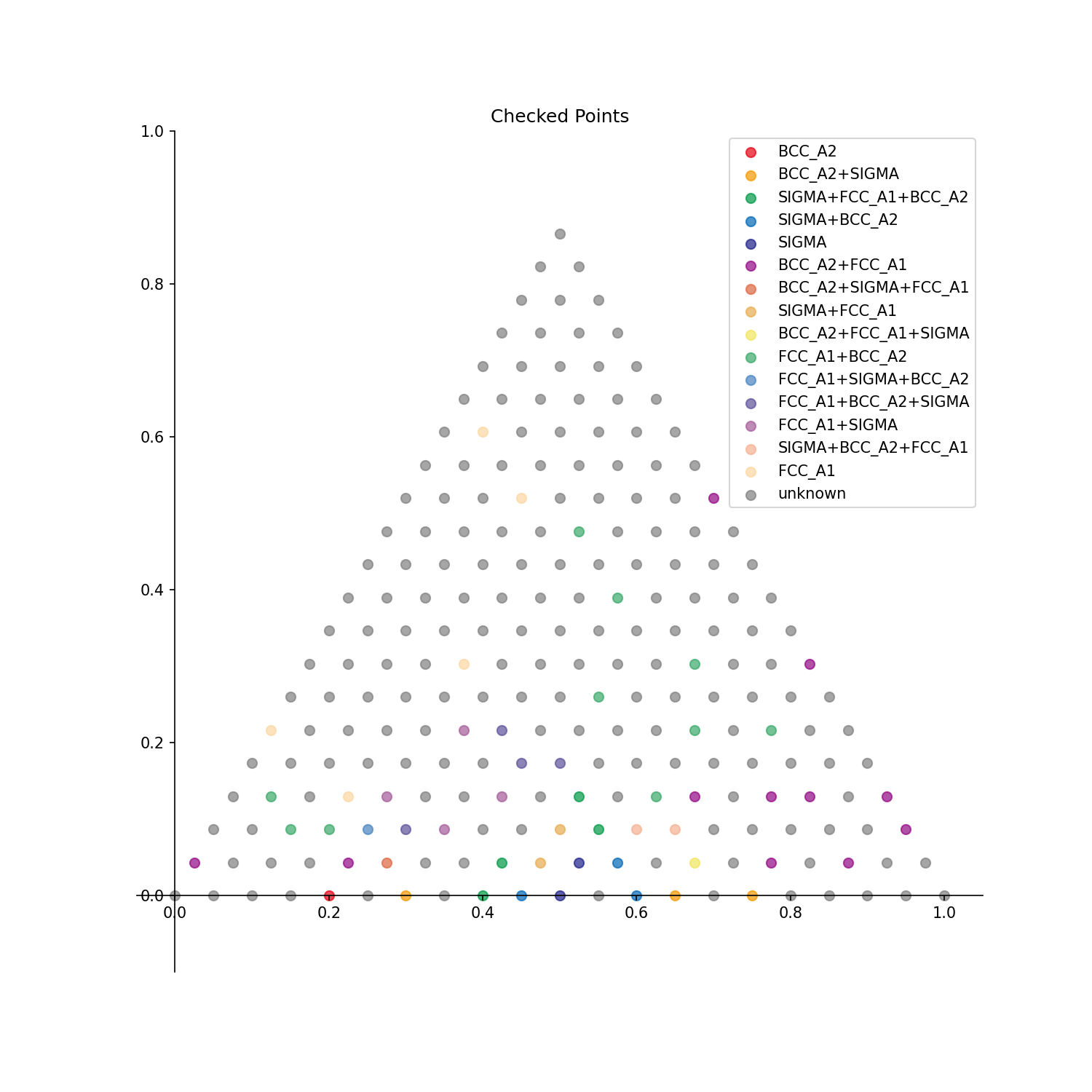
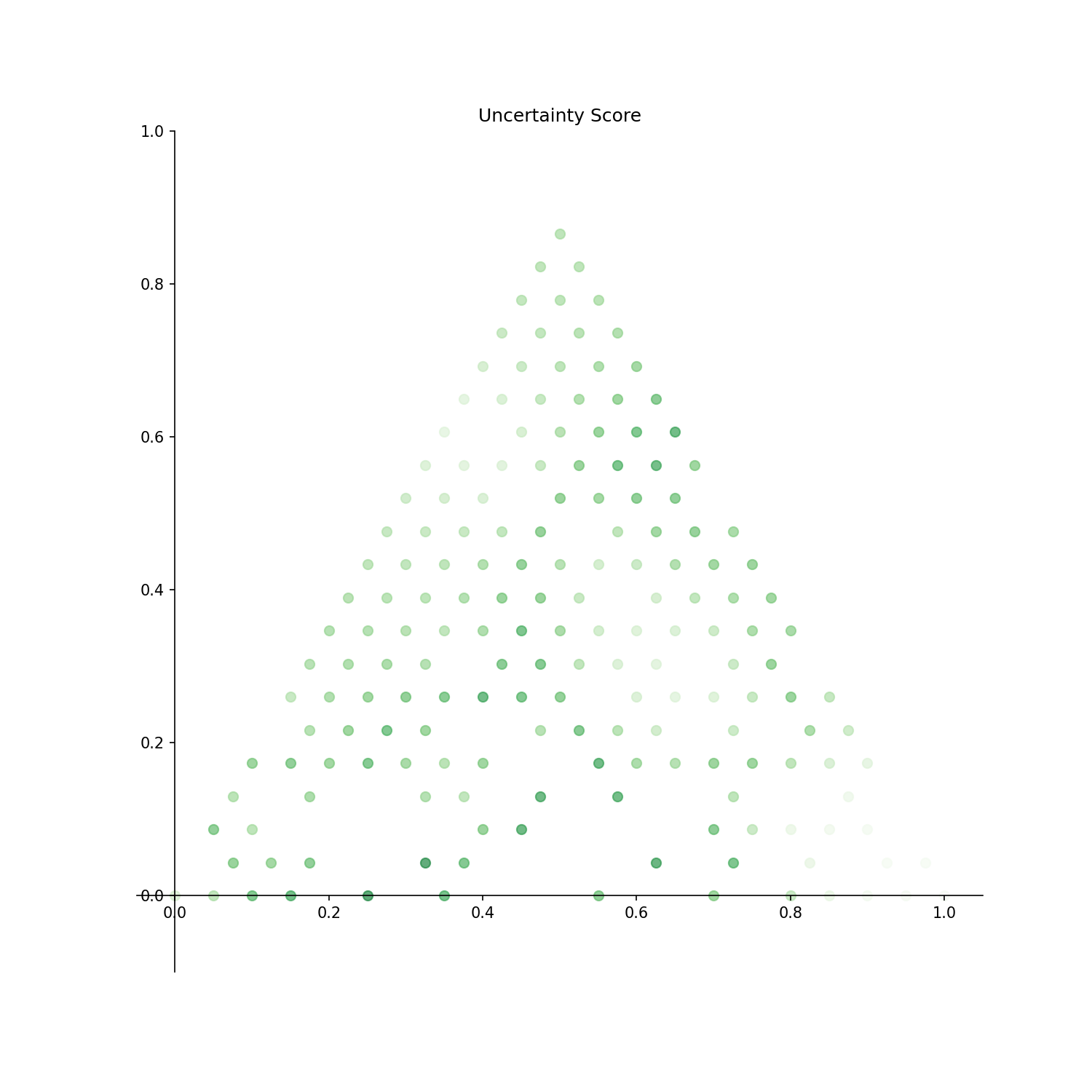
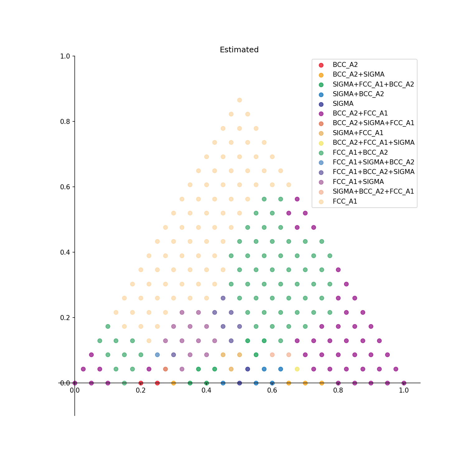
The following three figures are output in succession.
Checked Points: Points with already identified phases are displayed.
Uncertainty Score: Uncertainty score for each point is displayed.
Estimated: Estimated phase diagram is displayed.
In addition, below the code of proposals_index = pdc.proposals , the standard output about the proposal points is obtained as follows.
proposal_index: [5, 27, 33, 49, 68]
proposal_X: [[0.0, 0.75, 0.25], [0.05, 0.65, 0.3], [0.05, 0.35, 0.6], [0.1, 0.5, 0.4], [0.15, 0.45, 0.4]]
proposal_us: [0.7709398033192086, 0.7544588069243133, 0.6973660798457375, 0.672971896254403, 0.6686665138608043]
belonging_index_BCC_A2: [3, 5, 24, 2, 23]
belonging_X_BCC_A2: [[0.0, 0.85, 0.15], [0.0, 0.75, 0.25], [0.05, 0.8, 0.15], [0.0, 0.9, 0.1], [0.05, 0.85, 0.1]]
belonging_probability_BCC_A2: [0.3429449861197492, 0.22906019668079136, 0.22780732387481817, 0.16103851775328806, 0.14859411204017348]
belonging_index_BCC_A2+SIGMA: [14, 7, 16, 35, 5]
belonging_X_BCC_A2+SIGMA: [[0.0, 0.3, 0.7], [0.0, 0.65, 0.35], [0.0, 0.2, 0.8], [0.05, 0.25, 0.7], [0.0, 0.75, 0.25]]
belonging_probability_BCC_A2+SIGMA: [0.5084664081602635, 0.28798785026363194, 0.27569943113302103, 0.2723156235415327, 0.2279684961916743]
belonging_index_SIGMA+FCC_A1+BCC_A2: [28, 7, 70, 48, 87]
belonging_X_SIGMA+FCC_A1+BCC_A2: [[0.05, 0.6, 0.35], [0.0, 0.65, 0.35], [0.15, 0.35, 0.5], [0.1, 0.55, 0.35], [0.2, 0.35, 0.45]]
belonging_probability_SIGMA+FCC_A1+BCC_A2: [0.41641112113329276, 0.3728917200950976, 0.3463926061024242, 0.27514637238539996, 0.261158293406579]
belonging_index_SIGMA+BCC_A2: [11, 33, 28, 70, 49]
belonging_X_SIGMA+BCC_A2: [[0.0, 0.45, 0.55], [0.05, 0.35, 0.6], [0.05, 0.6, 0.35], [0.15, 0.35, 0.5], [0.1, 0.5, 0.4]]
belonging_probability_SIGMA+BCC_A2: [0.4564878867105817, 0.30263392015426255, 0.024008972043743384, 0.021434082521362623, 0.021049644410128583]
belonging_index_SIGMA: [11, 49, 33, 68, 70]
belonging_X_SIGMA: [[0.0, 0.45, 0.55], [0.1, 0.5, 0.4], [0.05, 0.35, 0.6], [0.15, 0.45, 0.4], [0.15, 0.35, 0.5]]
belonging_probability_SIGMA: [0.4390658028550059, 0.026249838699062628, 0.014755934814926938, 0.010435952482010182, 0.007072722883750504]
belonging_index_BCC_A2+FCC_A1: [40, 20, 39, 19, 58]
belonging_X_BCC_A2+FCC_A1: [[0.05, 0.0, 0.95], [0.0, 0.0, 1.0], [0.05, 0.05, 0.9], [0.0, 0.05, 0.95], [0.1, 0.05, 0.85]]
belonging_probability_BCC_A2+FCC_A1: [0.9794365586180334, 0.9754613868466422, 0.9745978351147191, 0.971462452609113, 0.963904881503319]
belonging_index_BCC_A2+SIGMA+FCC_A1: [5, 27, 7, 28, 24]
belonging_X_BCC_A2+SIGMA+FCC_A1: [[0.0, 0.75, 0.25], [0.05, 0.65, 0.3], [0.0, 0.65, 0.35], [0.05, 0.6, 0.35], [0.05, 0.8, 0.15]]
belonging_probability_BCC_A2+SIGMA+FCC_A1: [0.22508194319872216, 0.16911835513190335, 0.0763326785917378, 0.04446756734348071, 0.012293537080480565]
belonging_index_SIGMA+FCC_A1: [49, 68, 48, 11, 28]
belonging_X_SIGMA+FCC_A1: [[0.1, 0.5, 0.4], [0.15, 0.45, 0.4], [0.1, 0.55, 0.35], [0.0, 0.45, 0.55], [0.05, 0.6, 0.35]]
belonging_probability_SIGMA+FCC_A1: [0.327028103745597, 0.20879579727515543, 0.08199753318407586, 0.03698335729588441, 0.027629089037503673]
belonging_index_BCC_A2+FCC_A1+SIGMA: [14, 35, 54, 33, 55]
belonging_X_BCC_A2+FCC_A1+SIGMA: [[0.0, 0.3, 0.7], [0.05, 0.25, 0.7], [0.1, 0.25, 0.65], [0.05, 0.35, 0.6], [0.1, 0.2, 0.7]]
belonging_probability_BCC_A2+FCC_A1+SIGMA: [0.2818915371917155, 0.23520760088877765, 0.20596735819215564, 0.15735127720827985, 0.094689344987573]
belonging_index_FCC_A1+BCC_A2: [121, 135, 148, 122, 120]
belonging_X_FCC_A1+BCC_A2: [[0.3, 0.2, 0.5], [0.35, 0.2, 0.45], [0.4, 0.2, 0.4], [0.3, 0.15, 0.55], [0.3, 0.25, 0.45]]
belonging_probability_FCC_A1+BCC_A2: [0.8322472777083684, 0.8221340993971477, 0.8002307618798112, 0.797664402594447, 0.784769760536253]
belonging_index_FCC_A1+SIGMA+BCC_A2: [81, 5, 65, 62, 24]
belonging_X_FCC_A1+SIGMA+BCC_A2: [[0.2, 0.65, 0.15], [0.0, 0.75, 0.25], [0.15, 0.6, 0.25], [0.15, 0.75, 0.1], [0.05, 0.8, 0.15]]
belonging_probability_FCC_A1+SIGMA+BCC_A2: [0.028945840490463882, 0.028515902638765824, 0.024011902210446447, 0.02312600262738925, 0.02156548592795092]
belonging_index_FCC_A1+BCC_A2+SIGMA: [102, 117, 84, 103, 68]
belonging_X_FCC_A1+BCC_A2+SIGMA: [[0.25, 0.4, 0.35], [0.3, 0.4, 0.3], [0.2, 0.5, 0.3], [0.25, 0.35, 0.4], [0.15, 0.45, 0.4]]
belonging_probability_FCC_A1+BCC_A2+SIGMA: [0.6109220585078707, 0.4105500666597589, 0.37487447088734216, 0.37452268512936004, 0.33133348613919567]
belonging_index_FCC_A1+SIGMA: [66, 83, 65, 82, 84]
belonging_X_FCC_A1+SIGMA: [[0.15, 0.55, 0.3], [0.2, 0.55, 0.25], [0.15, 0.6, 0.25], [0.2, 0.6, 0.2], [0.2, 0.5, 0.3]]
belonging_probability_FCC_A1+SIGMA: [0.6516583590609779, 0.6208135568903499, 0.5986016823494428, 0.5502934531848476, 0.5177065740489881]
belonging_index_SIGMA+BCC_A2+FCC_A1: [33, 70, 54, 88, 35]
belonging_X_SIGMA+BCC_A2+FCC_A1: [[0.05, 0.35, 0.6], [0.15, 0.35, 0.5], [0.1, 0.25, 0.65], [0.2, 0.3, 0.5], [0.05, 0.25, 0.7]]
belonging_probability_SIGMA+BCC_A2+FCC_A1: [0.29954454085365223, 0.18113174228070997, 0.18039040498458211, 0.07334520526507098, 0.061454313319613256]
belonging_index_FCC_A1: [203, 210, 196, 197, 195]
belonging_X_FCC_A1: [[0.7, 0.3, 0.0], [0.75, 0.25, 0.0], [0.65, 0.3, 0.05], [0.65, 0.25, 0.1], [0.65, 0.35, 0.0]]
belonging_probability_FCC_A1: [0.8486182900941895, 0.832701029603124, 0.8210606957416035, 0.8148741219420823, 0.785430794433471]
Next, we will look at the results while using the web application version.
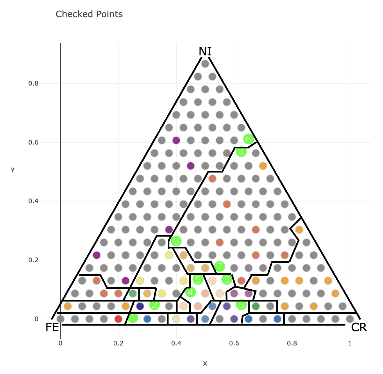
For the input data used as an example here, the complete phase diagram is known and the phase diagram is as follows. I drew this with a web application.
The phase boundary of this phase diagram is shown as follows.
proposal_index and proposal_X outputed by the Python code are the proposal points for the next experiment.
Under the same conditions, when 10 candidate points are calculated on the web application, green circle numbers are output as proposed points.
We can see that the same points are proposed as candidates for the next experiment in the Python version and the web application version.

Furthermore, when the figure of this proposed point and the phase boundary of the complete phase diagram are overlaid for comparison, it can be seen that the proposed points are located near the phase boundary, as shown below. In other words, the phase boundary can be determined accurately by conducting experiments according to these proposals.
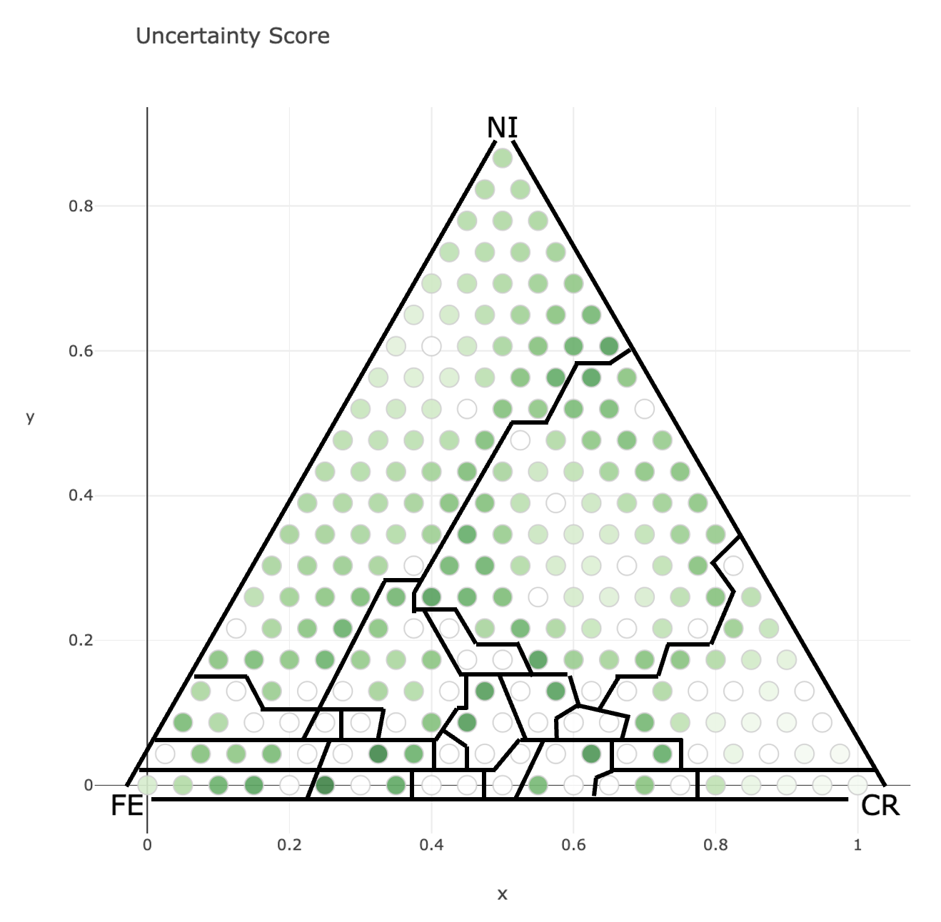
The distribution of uncertainty scores with the phase boundaries of the complete phase diagram is as follows.
In the web application version, we can obtain the experimental conditions with a high probability of belonging to each phase as follows.
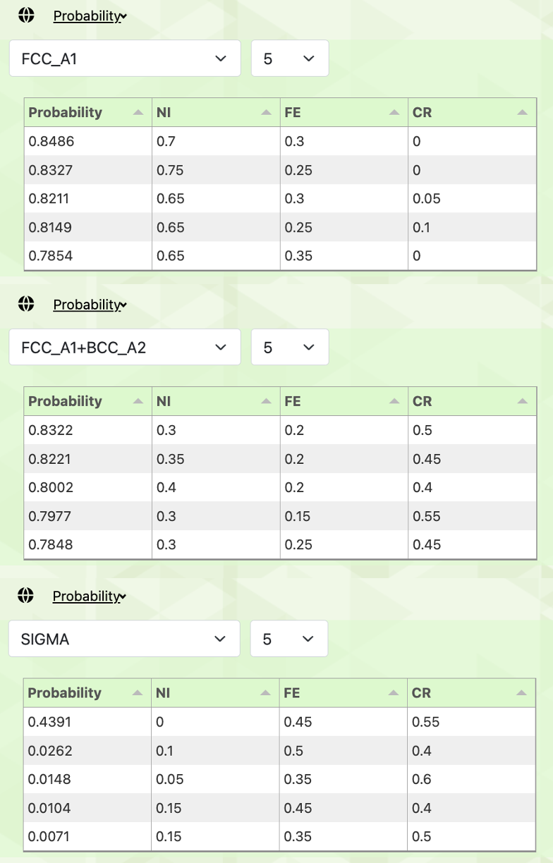
These correspond to belonging_index, belonging_X, and belonging_probability in the standard output of the Python version.
Inputting as an array
Data can also be input as an array when page_type is specified.
An array corresponding to the one specified in page_type is inputed as follows.
pdc  = pdc_sampler(page_type = "ternary_section",
                   estimation = "LP",
                   sampling = "LC",
                   proposal = 1)

X = np.array([
    [0.00,1.00,0.00],
    [0.00,0.50,0.50],
    [0.00,0.00,1.00],
    [0.50,0.50,0.00],
    [0.50,0.00,0.50],
    [1.00,0.00,0.00],
    ])

y = np.array([-1,-1,0,1,2,2])

pdc.fit(X,y)
pdc.us()

plot_out(pdc)
X: All candidate points in the discretized phase diagram are described. It can handle arbitrary dimensions.y: The phase index is putted in order from 0 at the point where the phase is already identified. For the points where the phase is not identified, the phase index -1 is specified.
The output result is as follows.
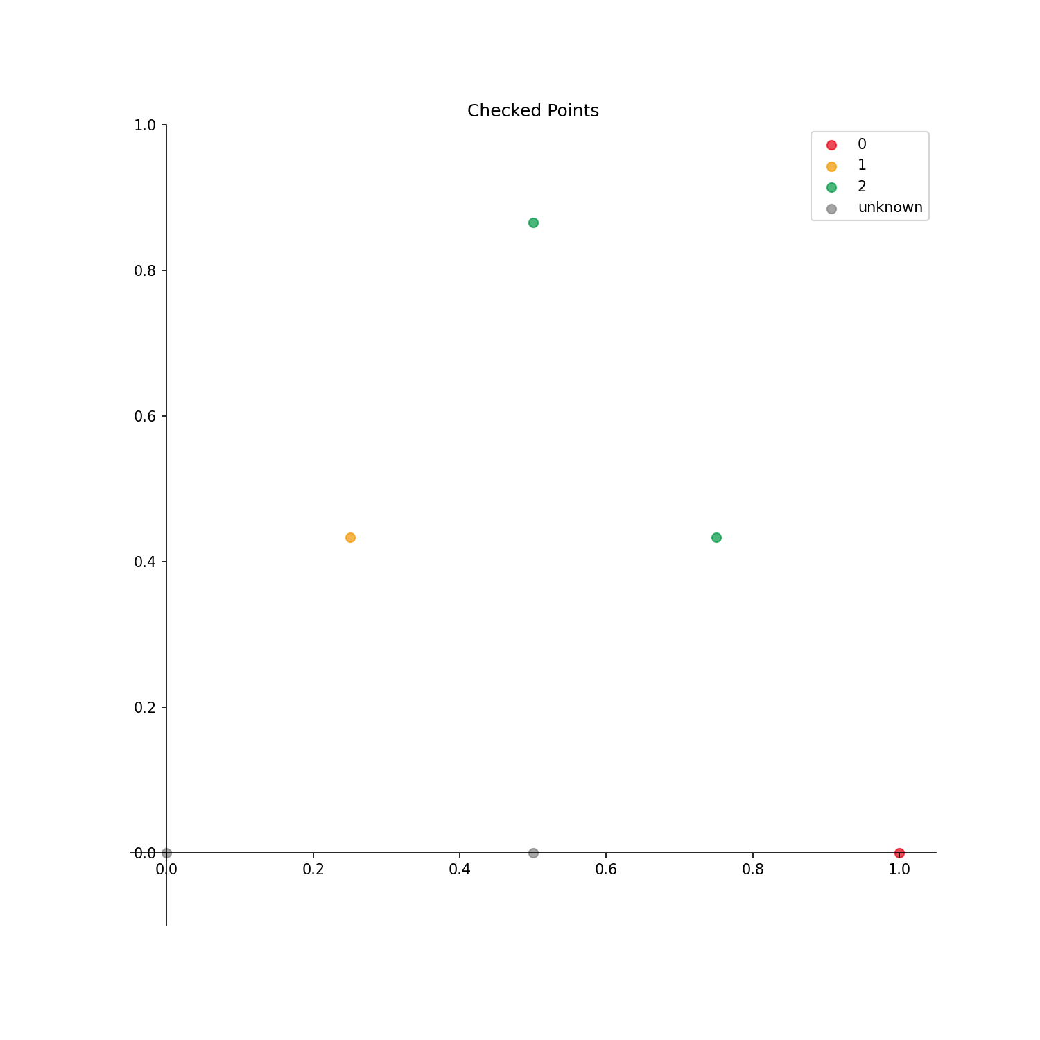
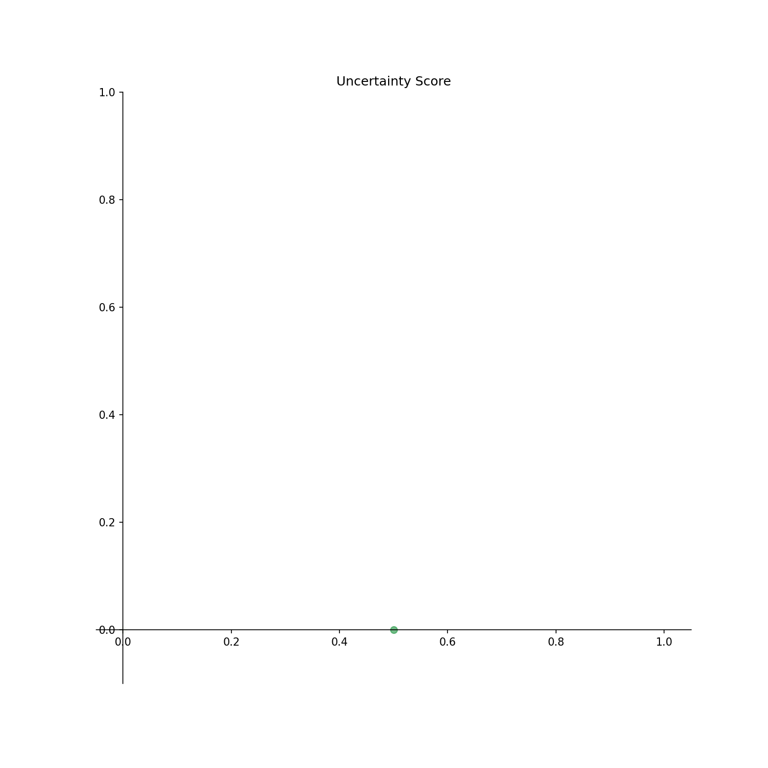
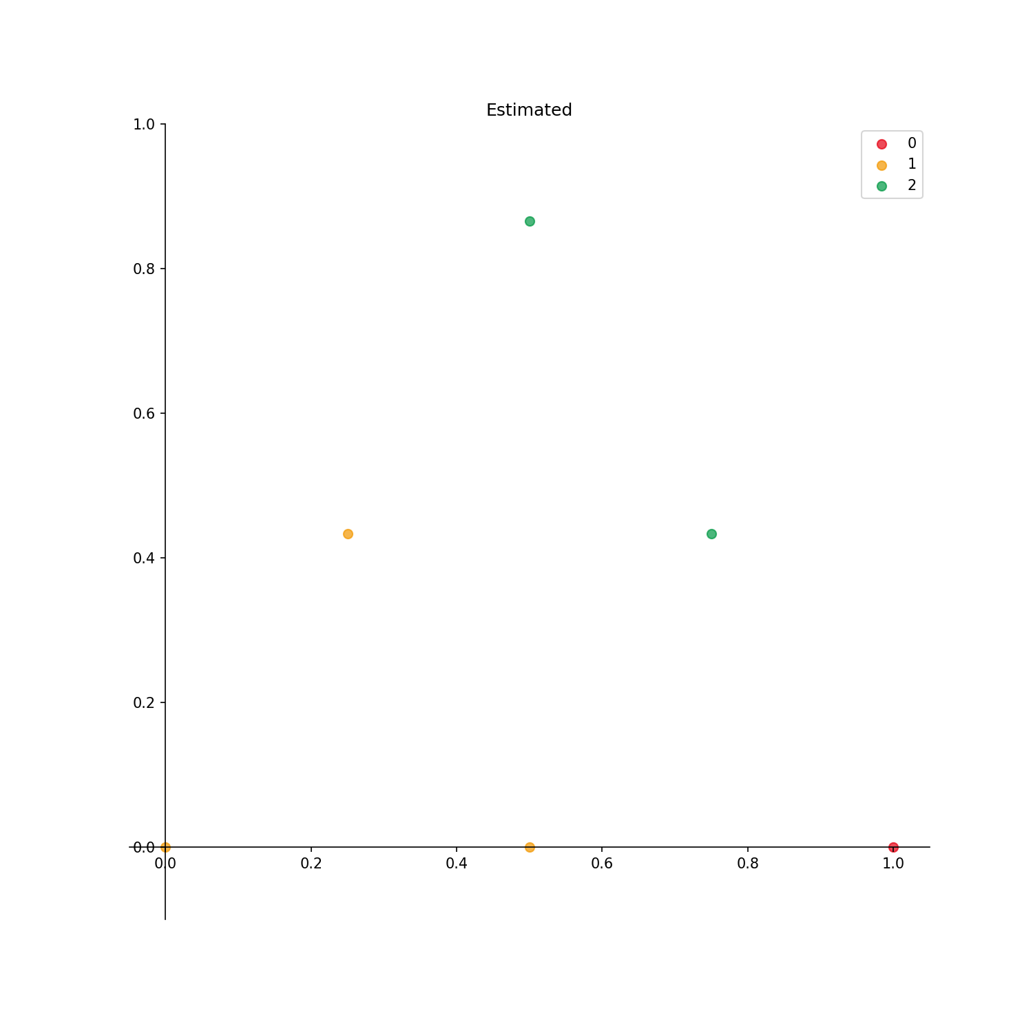
If no label is specified, a label is automatically generated with a serial number starting from 0 as shown in the above figure.
Specifying a label
When inputting as an array, any label can be input.
If we want to enter an arbitrary label, phase_id_option can be used as follows.
pdc  = pdc_sampler(page_type = "ternary_section",
                   estimation = "LP",
                   sampling = "LC",
                   phase_id_option = {"a":0,"b":1,"c":2},
                   proposal = 1
                   )

X = np.array([
    [0.00,1.00,0.00],
    [0.00,0.50,0.50],
    [0.00,0.00,1.00],
    [0.50,0.50,0.00],
    [0.50,0.00,0.50],
    [1.00,0.00,0.00],
    ])

y = np.array([-1,-1,0,1,2,2])

pdc.fit(X,y)
pdc.us()

plot_out(pdc)
phase_id_option: Write {“a”: 0 ,”b”: 1 ,”c”: 2 } to correspond to 0, 1, 2 in the arrayy.
The output result is as follows.


Output options
AIPHAD can output three types of figures.
Checked_points: Points with already identified phases are displayed.Uncertainty_score: Uncertainty score for each point is displayed.Estimated: Estimated phase diagram is displayed.
There are two ways to output figures.
Display the output of the figure on the desktop.
Save the figure as an image.
To output the figure, plot_out(pdc) is used.
If no option is specified, the figure is displayed on the desktop by default.
An example is shown below.
pdc  = pdc_sampler(input_data = "example_ternary_iso.csv",
                   page_type = "ternary_section",
                   estimation = "LP",
                   sampling = "LC",
                   proposal = 3
                   )

pdc.fit()
pdc.us()

plot_out(pdc)
To save the figure as an image, the following options is used.
pdc  = pdc_sampler(input_data = "example_ternary_iso.csv",
                   page_type = "ternary_section",
                   estimation = "LP",
                   sampling = "LC",
                   proposal = 3
                   )

pdc.fit()
pdc.us()

plot_out(pdc, elev_num = 30, azim_num = 45, save_fig = True, extension = "png", directory_name = "./out1")
An explanation of each option is as follows.
save_fig: To save the figure as an image, “True” is specified, and “False” is specified to output the figure to the desktop.elev_num: For 3D figures, we can specify the elevation angle relative to the z-axis.azim_num: For 3D figures, we can specify the azimuth along the x and y axes.extension: We can specify the extension of the image. We can specify png, jpg, or pdf.directory_name: The save directory is specified. A folder with the name specified bypage_typewill be created in this folder, and the figure will be output in that folder.